13.3. Collaborative Filtering
The collaborative filtering method replies on an interaction matrix between users and items, known as the rating matrix. Imagine this matrix as an m-by-n grid, where rows represent users, columns represent items.
Within this matrix, some entries are known, which could be explicit or implicit feedback. Explicit feedback might be direct ratings, such as a user’s rating of a movie on Netflix on a scale from one to five, signaling clear preferences. Implicit feedback could come from user behaviors such as clicking on an item or spending time viewing a particular movie, providing subtle clues about their interests.
Constructing this matrix, however, is far from trivial. Challenges arise in distinguishing between a user’s disinterest in an item and mere unawareness of it. Missing entries don’t always mean disliking; they could indicate a lack of exposure. This ambiguity is just one of the hurdles in developing effective recommendation systems.
Assuming we have this interaction matrix, denoted by R, with some entries missing (indicated by question marks), the goal of a recommender system is to fill in the blanks, predicting user preferences for items they haven’t interacted with. This task is akin to matrix completion, a term you’ll often encounter when delving into the mechanics of recommendation systems.
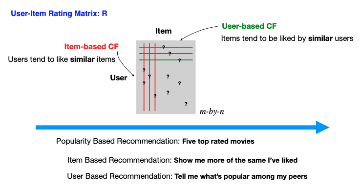
Collaborative filtering splits into two primary methods: User-based and Item-based.
- User-based CF
This approach posits that similar users will like similar items. If User A liked an item and User B has a similar profile to User A, it’s likely that User B will also like that item. The challenge lies in defining what makes users similar, which we will explore further.
- Item-based CF
Conversely, this method assumes users will like items similar to those they have already liked. If User A liked Item X, and Item Y is similar to Item X, then User A is likely to like Item Y as well.
Crucial to collaborative filtering is the notion of similarity. We need to determine how to quantify the resemblance between users or items, even with incomplete data. Some of the most commonly used similarity metrics include:
- Jaccard Similarity:
Ideal for binary data, it compares users based on the items they have both interacted with, or compare items based on shared users.
\[\frac{|A \cap B|}{|A \cup B|}, \quad \text{ where } A, B \text{ are two sets}\]
- Cosine Similarity:
This measures the cosine of the angle between two vectors in an n-dimensional space. Missing values are ignored or equivalently treated as zeros.
\[\frac{u^t v}{\| u\| \cdot \| v\|}, \quad \text{ where } u, v \text{ are two vectors}\]
- Centered Cosine Similarity (Pearson Correlation):
A variation of cosine similarity first normalizes around a user’s (or item’s) average rating by subtracting the mean of the observed values.
\[\frac{(u - \bar{u})^t (v - \bar{v})}{\| u - \bar{u} \| \cdot \| v- \bar{v} \|}, \quad \text{ where } u, v \text{ are two vectors}\]
When working with cosine-based similarity measures, it’s important to consider a couple of Key Issues:
Cosines (or correlation coefficients) fall within the range [-1, 1], while similarity measures are typically expected to be within the range [0, 1]. To bridge this gap, it’s customary to define similarity as (1 + cos)/2.
The measures are computed based on the shared, non-missing elements between two entities. For example, for users u and v, the calculation relies on ratings for items that they have both rated. This implies that in the calculation the length of vector u can vary depending on whether we are computing the similarity between u and v1 or the similarity between u and v2. It’s worth noting that it’s common to obtain a similarity of 1 between two users if they have rated only one shared item.
When it comes to Centered Cosine similarity,
one approach is to confine all calculations, including centering, to the shared, non-missing elements between two entities This aligns with the pairwise.complete.obs method in the R command cor. However, some may find such computed similarity less comparable or reasonable.
An alternative approach for calculating Centered Cosine similarity involves first centering each user’s ratings to eliminate user bias and then computing the cosine similarity. For example, if user u has rated 10 movies, and 3 of those movies are also rated by user v, the calculation during the centering stage takes into account all 10 ratings, whereas the cosine calculation considers only the shared 3 ratings. In contrast, in the centered cosine similarity calculation mentioned above, all computations, including centering, are restricted to the three shared ratings.
Additionally, when calculating centered cosine similarity, it’s crucial to be mindful of a potential issue related to the denominator: \(\| u - \bar{u} \|.\) This denominator can become zero when all non-NA (non-missing) elements of u are constant.
In summary, with a well-constructed R matrix and a thoughtful selection of similarity measures, collaborative filtering can make educated predictions, catering to the diverse tastes of their audience.