9.7. Summary
In Discriminant Analysis, we initially find the optimal decision rule for classification based on conditional probabilities. The approach in Discriminant Analysis is to estimate these probabilities by following a different factorization method.
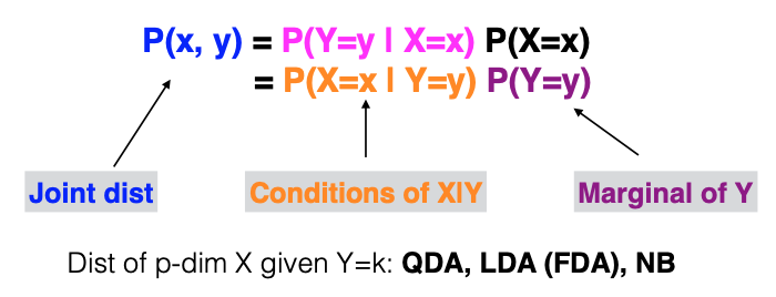
We estimate the margins of Y and the conditional distribution of X given Y and combine them to obtain the joint distribution. From this joint distribution, we can derive the marginal distribution. Depending on how we model the conditional distribution of X given Y, several Discriminant Analysis methods like Quadratic Discriminant Analysis (QDA), Linear Discriminant Analysis (LDA), or Naive Bayes can be employed.
Discriminant Analysis is conceptually straightforward and is effective for low-dimensional problems, particularly QDA and LDA. However, it may not be the most efficient method for building classifiers.
Let’s take a closer look at binary LDA, where k can take only two different values, and the discriminant function or decision function is a linear function of \(x\) with coefficients determined by \((\Sigma, \mu_k, \pi_k)\).
In binary classification, our main concern is the difference between \(d_1(x)\) and \(d_2(x)\), which is a linear function of \(x\):
So what truly matters is the linear function’s p-dimensional coefficient vector \(\boldsymbol{\beta}\), along with the intercept \(\beta_0\). However, LDA estimates these p + 1 parameters using a much larger collection of parameters, including a p-by-p covariance matrix \(\Sigma\), two p-dimensional vectors \(\mu_1\) and \(\mu_2\), and a mixing weight \(\pi_1\).
In the upcoming weeks, we’ll delve into methods that directly learn the conditional probability/decision boundary as a function of \(x\), such as logistic regression or tree models, which directly learn probabilities, or support vector machines (SVMs), which directly learn the decision boundary.